Link: Linear regresssion R
library(dplyr)
# Get data
mouse.data <- data.frame(
  weight=c(0.9, 1.8, 2.4, 3.5, 3.9, 4.4, 5.1, 5.6, 6.3),
  size=c(1.4, 2.6, 1.0, 3.7, 5.5, 3.2, 3.0, 4.9, 6.3))

## plot a x/y scatter plot with the data
plot(mouse.data$weight, mouse.data$size)

## create a "linear model" - that is, do the regression
## where y = intercept + slope * x
mouse.regression <- lm(size ~ weight, data=mouse.data)

## add the regression line to our x/y scatter plot
abline(mouse.regression, col="blue")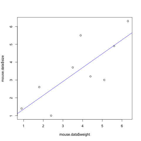
Interpret the results
## generate a summary of the regression
summary(mouse.regression)
Call:
lm(formula = size ~ weight, data = mouse.data)

Residuals:
    Min      1Q  Median      3Q     Max
-1.5482 -0.8037  0.1186  0.6186  1.8852

Coefficients:
            Estimate Std. Error t value Pr(>|t|)
(Intercept)   0.5813     0.9647   0.603   0.5658
weight        0.7778     0.2334   3.332   0.0126 *
---
Signif. codes:  0 ‘***’ 0.001 ‘**’ 0.01 ‘*’ 0.05 ‘.’ 0.1 ‘ ’ 1

Residual standard error: 1.19 on 7 degrees of freedom
Multiple R-squared:  0.6133,	Adjusted R-squared:  0.558
F-statistic: 11.1 on 1 and 7 DF, p-value: 0.01256- Call: This just show the function that was called
- Residuals: Same as the one in box plot
- Coefficients: When looking at the p-value in the coefficients table (shown as
Pr(>|t|)), generally the one in intercept does not matter. On the other hand, we want the p-value of slope (weight in this example) to be < 0.05 in order to be statistically significant. - Residual standard error: The square root of the denominator in the equation for F-value
- Multiple R-squared: Equals R-squared
- Adjusted R-squared: R-squared scaled by the number of parameters
- F-statistic(F-value): the value of F, DF = degree of freedom
- P-value: in this case p-value < 0.05, meaning the x(weight) gives us a reliable estimate for y(size)