Multiple regression in R

Link: Multiple regression R Linear regression in R

Check the full code in github repo.

Do multiple regression in R §

Plot the basic correlation §

library(dplyr)
mouse.data <- data.frame(
  size = c(1.4, 2.6, 1.0, 3.7, 5.5, 3.2, 3.0, 4.9, 6.3),
  weight = c(0.9, 1.8, 2.4, 3.5, 3.9, 4.4, 5.1, 5.6, 6.3),
  tail = c(0.7, 1.3, 0.7, 2.0, 3.6, 3.0, 2.9, 3.9, 4.0))
 
plot(mouse.data)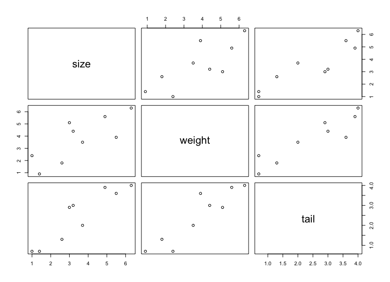

Interpret the graph §

Identify the correlation by eye-balling:

• Both weight and tail are correlated with size.
• weight and tail are also correlated - so we might not need both

Fit a plane to the data §

Use ”+” sign in lm() to indicate multiple parameters.

multiple.regression <- lm(size ~ weight + tail, data=mouse.data)

Use summary() to interpret the results §

Note: since we are using multiple regression, the adjusted R-squared would be more meaningful.

Call:
lm(formula = size ~ weight + tail, data = mouse.data)

Residuals:
     Min       1Q   Median       3Q      Max
-0.99928 -0.38648 -0.06967  0.34454  1.07932

Coefficients:
            Estimate Std. Error t value Pr(>|t|)
(Intercept)   0.7070     0.6510   1.086   0.3192
weight       -0.3293     0.3933  -0.837   0.4345
tail          1.6470     0.5363   3.071   0.0219 *
---
Signif. codes:  0 ‘***’ 0.001 ‘**’ 0.01 ‘*’ 0.05 ‘.’ 0.1 ‘ ’ 1

Residual standard error: 0.8017 on 6 degrees of freedom
Multiple R-squared:  0.8496,	Adjusted R-squared:  0.7995
F-statistic: 16.95 on 2 and 6 DF,  p-value: 0.003399

How to compare between multiple vs linear regression §

We can do so by comparing the coefficient table with simple linear regression:

The lines of x variables represents the results of multipe regression while comparing with simple linear regression without it.

e.g. The weight line compares the multipel regression y = n + a*weight + b*tail vs simple regression y = n + b*tail. In this case, p-value > 0.05, so weight + tail is not significantly better(important) than using tail alone to predict size, meaning we can get rid of weight in the model.